39 change data labels in excel chart

Edit titles or data labels in a chart - support.microsoft.com Change the position of data labels On a chart, do one of the following: To reposition all data labels for an entire data series, click a data label once to... To reposition all data labels for an entire data series, click a data label once to select the data series. To reposition a specific data ... How to Edit Pie Chart in Excel (All Possible Modifications) 7. Change Data Labels Position. Just like the chart title, you can also change the position of data labels in a pie chart. Follow the steps below to do this. 👇. Steps: Firstly, click on the chart area. Following, click on the Chart Elements icon. Subsequently, click on the rightward arrow situated on the right side of the Data Labels option ...

Add data labels and callouts to charts in Excel 365 | EasyTweaks.com Excel also gives you the option of formatting the data labels to suit your desired look if you don't like the default. To make changes to the data labels, right-click within the chart and select the "Format Labels" option. Some of the formatting options you will have include; changing the label position, changing its alignment angle, and many more.

Change data labels in excel chart

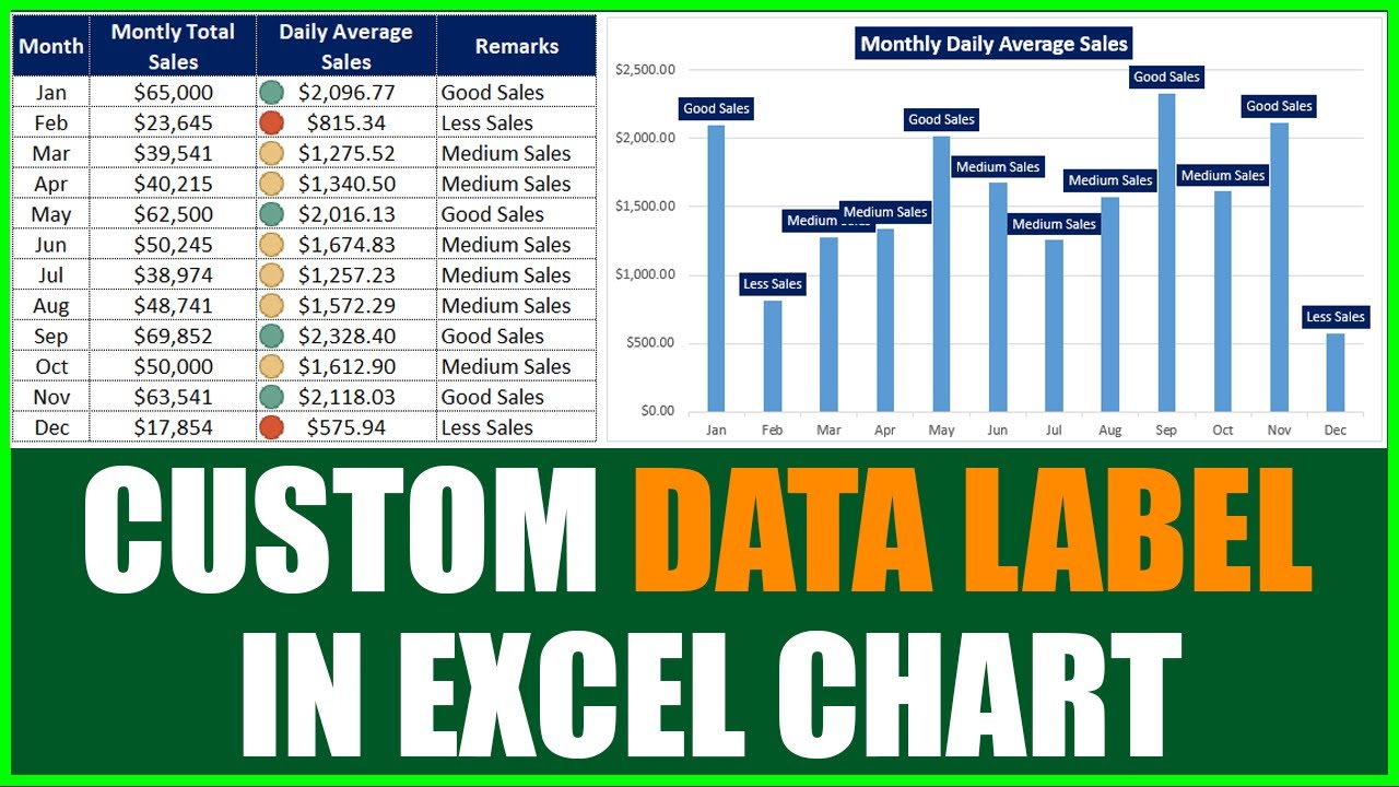
Custom Chart Data Labels In Excel With Formulas Follow the steps below to create the custom data labels. Select the chart label you want to change. In the formula-bar hit = (equals), select the cell reference containing your chart label's data. In this case, the first label is in cell E2. Finally, repeat for all your chart laebls. How to add data labels from different column in an Excel chart? This method will guide you to manually add a data label from a cell of different column at a time in an Excel chart. 1. Right click the data series in the chart, and select Add Data Labels > Add Data Labels from the context menu to add data labels. 2. Click any data label to select all data labels, and then click the specified data label to select it only in the chart. Format Data Labels in Excel- Instructions - TeachUcomp, Inc. To do this, click the "Format" tab within the "Chart Tools" contextual tab in the Ribbon. Then select the data labels to format from the "Chart Elements" drop-down in the "Current Selection" button group. Then click the "Format Selection" button that appears below the drop-down menu in the same area.

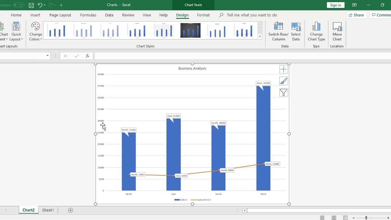
Change data labels in excel chart. Change axis labels in a scatter chart Excel Archives - Data Cornering Tag: Change axis labels in a scatter chart Excel DataViz Excel. How to add text labels on Excel scatter chart axis How to Use Cell Values for Excel Chart Labels Select the chart, choose the "Chart Elements" option, click the "Data Labels" arrow, and then "More Options." Uncheck the "Value" box and check the "Value From Cells" box. Select cells C2:C6 to use for the data label range and then click the "OK" button. The values from these cells are now used for the chart data labels. How to Rename a Data Series in Microsoft Excel To do this, right-click your graph or chart and click the "Select Data" option. This will open the "Select Data Source" options window. Your multiple data series will be listed under the "Legend Entries (Series)" column. To begin renaming your data series, select one from the list and then click the "Edit" button. How to create Custom Data Labels in Excel Charts Right click on any data label and choose the callout shape from Change Data Label Shapes option. Now adjust each data label as required to avoid overlap. Put solid fill color in the labels Finally, click on the chart (to deselect the currently selected label) and then click on a data label again (to select all data labels).

How to Add Data Labels in Excel - Excelchat | Excelchat In Excel 2013 and the later versions we need to do the followings; Click anywhere in the chart area to display the Chart Elements button Figure 5. Chart Elements Button Click the Chart Elements button > Select the Data Labels, then click the Arrow to choose the data labels position. Figure 6. How to Add Data Labels in Excel 2013 Figure 7. change Excel scatter chart horizontal axis labels Archives - Data Cornering Tag: change Excel scatter chart horizontal axis labels. DataViz Excel. How to add text labels on Excel scatter chart axis. by Janis Sturis July 11, 2022 Comments 0. Categories. Change the format of data labels in a chart To format data labels, select your chart, and then in the Chart Design tab, click Add Chart Element > Data Labels > More Data Label Options. Click Label Options and under Label Contains, pick the options you want. To make data labels easier to read, you can move them inside the data points or even outside of the chart. Adding Data Labels To An Excel Chart | MyExcelOnline In our example below, I add a Data Label to a column chart and then I format the data label using CTRL+1. I then select to custom format the numbers so it shows the values as thousands by adding a comma , after each zero and then showing the work k by adding "k" Example Custom Number Format: [$$-1004]#,##0 ,"k" ;- [$$-1004]#,##0 ,"k"

How To Add Data Labels In Excel | Nabludatel To format data labels in excel, choose the set of data labels to format. After inserting a chart in excel 2010 and earlier versions we need to do the followings to add data labels to the chart; How to Add Data Labels to an Excel 2010 Chart dummies from . When you select the "add labels" option, all the different portions of ... Excel Chart - Selecting and updating ALL data labels - Right-click a "point" in the series, which actually will be a bar piece - Choose add data labels - Right-click again and choose format data labels - Check series name - Uncheck value That's it…. You must log in or register to reply here. Excel contains over 450 functions, with more added every year. How do I customize axis labels in Excel? - Digglicious.com The chart uses text from your source data for axis labels. To change the label, you can change the text in the source data. How do I change the font of axis labels? In Horizontal (Category) Axis Labels, click Edit. In Axis label range, enter the labels you want to use, separated by commas. For example, type Quarter 1 ,Quarter 2,Quarter 3,Quarter 4. How to Change Excel Chart Data Labels to Custom Values? First add data labels to the chart (Layout Ribbon > Data Labels) Define the new data label values in a bunch of cells, like this: Now, click on any data label. This will select "all" data labels. Now click once again. At this point excel will select... Go to Formula bar, press = and point to the ...

How To Add Data Labels To A Chart in Microsoft Excel - YouTube

How to add and customize chart data labels - Get Digital Help Double press with left mouse button on with left mouse button on a data label series to open the settings pane. Go to tab "Label Options" see image to the right. This setting allows you to change the number formatting of the data labels. The image below shows numbers formatted as dates.

Show Trend Arrows in Excel Chart Data Labels | Excel, Chart, Excel tutorials

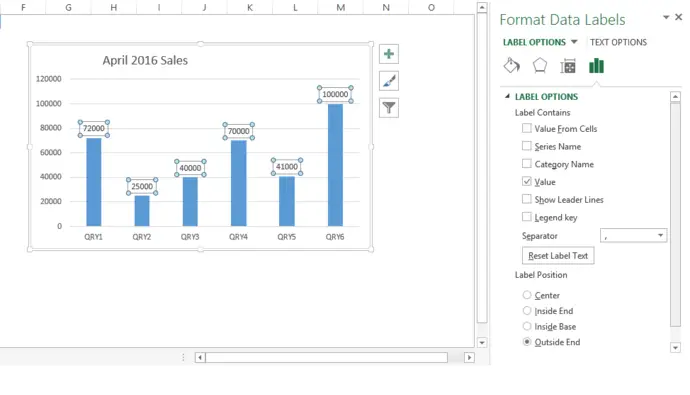
Excel charts: add title, customize chart axis, legend and data labels To change what is displayed on the data labels in your chart, click the Chart Elements button > Data Labels > More options… This will bring up the Format Data Labels pane on the right of your worksheet. Switch to the Label Options tab, and select the option (s) you want under Label Contains:

How to Add Data Labels in Excel - Excelchat | Excelchat

Excel Chart Data Labels-Modifying Orientation - Microsoft Community You can right click on the data label part then select Format Axis. Click on the Size & Properties tab then adjust the Text Direction or Custom Angle. Thanks, Mike Report abuse 7 people found this reply helpful · Was this reply helpful? Yes No

Do My Excel Blog: How to design a multiple clustered bar chart series in Excel

Excel resize chart title 6. Especially if using Excel to monitor, edit, share data, creating a circular chart will be very reasonable. By using a simple spreadsheet, today's article will show you how to. It also will reduce wasted white space on the charts. It's easy to do this in Excel. Right Click on the bars. Format data series. Series Options. Gap. You will see a ...

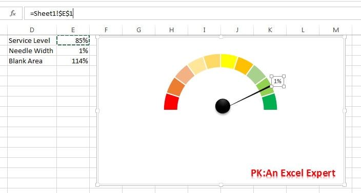
Speedometer Chart - PK: An Excel Expert

How to Customize Your Excel Pivot Chart Data Labels - dummies To add data labels, just select the command that corresponds to the location you want. To remove the labels, select the None command. If you want to specify what Excel should use for the data label, choose the More Data Labels Options command from the Data Labels menu. Excel displays the Format Data Labels pane.

Enable or Disable Excel Data Labels at the click of a button - How To - PakAccountants.com

Change the labels in an Excel data series | TechRepublic salary expenses, follow these steps: Select B15:D15. Click the Chart Wizard button in the Standard toolbar. Click Next. Click the Series tab. Click the Window Shade button in the Category (X) Axis ...

How to Add Data Labels to your Excel Chart in Excel 2013 - YouTube

Change the format of data labels in a chart Tip: To switch from custom text back to the pre-built data labels, click Reset Label Text under Label Options. To format data labels, select your chart, and then in the Chart Design tab, click Add Chart Element > Data Labels > More Data Label Options. Click Label Options and under Label Contains, pick the options you want.

Excel Charts | Real Statistics Using Excel

Modify Excel Chart Data Range | CustomGuide Click the Design tab. Click the Select Data button. Select the series you want to change under Legend Entries (Series). Click the Edit button. Type the label you want to use for the series in the Series name field. Click OK. Click OK again. The name is updated in the chart, but the worksheet data remains unchanged.

Pie Chart - PK: An Excel Expert

How to add or move data labels in Excel chart? - ExtendOffice Add or move data labels in Excel chart 1. Click the chart to show the Chart Elements button . 2. Then click the Chart Elements, and check Data Labels, then you can click the arrow to choose an option about the data...

How do I change the order of pie chart slices?

Add / Move Data Labels in Charts - Excel & Google Sheets We'll start with the same dataset that we went over in Excel to review how to add and move data labels to charts. Add and Move Data Labels in Google Sheets. Double Click Chart; Select Customize under Chart Editor; Select Series . 4. Check Data Labels. 5. Select which Position to move the data labels in comparison to the bars. Final Graph with Google Sheets. After moving the dataset to the center, you can see the final graph has the data labels where we want.

Formula Friday - Using Formulas To Add Custom Data Labels To Your Excel Chart - How To Excel At ...

Format Data Labels in Excel- Instructions - TeachUcomp, Inc. To do this, click the "Format" tab within the "Chart Tools" contextual tab in the Ribbon. Then select the data labels to format from the "Chart Elements" drop-down in the "Current Selection" button group. Then click the "Format Selection" button that appears below the drop-down menu in the same area.

Excel Course: Inserting Graphs

How to add data labels from different column in an Excel chart? This method will guide you to manually add a data label from a cell of different column at a time in an Excel chart. 1. Right click the data series in the chart, and select Add Data Labels > Add Data Labels from the context menu to add data labels. 2. Click any data label to select all data labels, and then click the specified data label to select it only in the chart.