41 how to add axis labels in excel bar graph

Excel charts: add title, customize chart axis, legend and ... When creating graphs in Excel, you can add titles to the horizontal and vertical axes to help your users understand what the chart data is about. To add the axis titles, do the following: Click anywhere within your Excel chart, then click the Chart Elements button and check the Axis Titles box. How to Add Gridlines in a Chart in Excel? 2 Easy Ways! Let us now see two ways to insert major and minor gridlines in Excel. Method 1: Using the Chart Elements Button to Add and Format Gridlines. The Chart Elements button appears to the right of your chart when it is selected. This button allows you to add, change or remove chart elements like the title, legend, gridlines, and labels.

How to Insert Axis Labels In An Excel Chart | Excelchat We will go to Chart Design and select Add Chart Element Figure 6 - Insert axis labels in Excel In the drop-down menu, we will click on Axis Titles, and subsequently, select Primary vertical Figure 7 - Edit vertical axis labels in Excel Now, we can enter the name we want for the primary vertical axis label.

How to add axis labels in excel bar graph

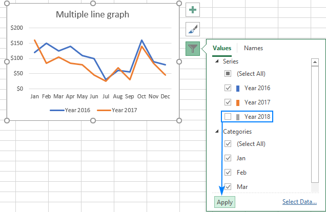
Move Horizontal Axis to Bottom – Excel & Google Sheets Moving X Axis to the Bottom of the Graph. Click on the X Axis; Select Format Axis . 3. Under Format Axis, Select Labels. 4. In the box next to Label Position, switch it to Low. Final Graph in Excel. Now your X Axis Labels are showing at the bottom of the graph instead of in the middle, making it easier to see the labels. How to Create a Bar Chart With Labels Inside Bars in Excel 7. In the chart, right-click the Series "# Footballers" Data Labels and then, on the short-cut menu, click Format Data Labels. 8. In the Format Data Labels pane, under Label Options selected, set the Label Position to Inside End. 9. Next, in the chart, select the Series 2 Data Labels and then set the Label Position to Inside Base. How to Add a Secondary Axis to an Excel Chart - HubSpot Step 3: Add your secondary axis. Under the "Start" tab, click on the graph at the bottom right showing a bar graph with a line over it. If that doesn't appear in the preview immediately, click on "More >>" next to the "Recommended charts" header, and you will be able to select it there. Make sure that "Use column A as headers" is checked at the ...

How to add axis labels in excel bar graph. How To Add Axis Labels In Excel - BSUPERIOR Add Title one of your chart axes according to Method 1 or Method 2. Select the Axis Title. (picture 6) Picture 4- Select the axis title Click in the Formula Bar and enter =. Select the cell that shows the axis label. (in this example we select X-axis) Press Enter. Picture 5- Link the chart axis name to the text Label Specific Excel Chart Axis Dates - My Online Training Hub Steps to Label Specific Excel Chart Axis Dates. The trick here is to use labels for the horizontal date axis. We want these labels to sit below the zero position in the chart and we do this by adding a series to the chart with a value of zero for each date, as you can see below: Note: if your chart has negative values then set the 'Date Label ... Add / Move Data Labels in Charts - Excel & Google Sheets Adding Data Labels Click on the graph Select + Sign in the top right of the graph Check Data Labels Change Position of Data Labels Click on the arrow next to Data Labels to change the position of where the labels are in relation to the bar chart Final Graph with Data Labels Change axis labels in a chart in Office In charts, axis labels are shown below the horizontal (also known as category) axis, next to the vertical (also known as value) axis, and, in a 3-D chart, next to the depth axis. The chart uses text from your source data for axis labels. To change the label, you can change the text in the source data.

Custom Axis Labels and Gridlines in an Excel Chart In Excel 2013, click the "+" icon to the top right of the chart, click the right arrow next to Data Labels, and choose More Options…. Then in all versions, choose the Label Contains option for Y Values and the Label Position option for Left. The labels are (temporarily) shaded yellow to distinguish them from the built-in axis labels. How to add axis label to chart in Excel? - ExtendOffice You can insert the horizontal axis label by clicking Primary Horizontal Axis Title under the Axis Title drop down, then click Title Below Axis, and a text box will appear at the bottom of the chart, then you can edit and input your title as following screenshots shown. 4. How to Create a Bar Chart With Labels Above Bars in Excel In the chart, right-click the Series "Dummy" data series and then, on the shortcut menu, click Add Data Labels. The chart should look like this: 14. In the chart, right-click the Series "Dummy" Data Labels and then, on the short-cut menu, click Format Data Labels. 15. Excel Chart Vertical Axis Text Labels • My Online Training Hub Click on the top horizontal axis and delete it. Hide the left hand vertical axis: right-click the axis (or double click if you have Excel 2010/13) > Format Axis > Axis Options: Set tick marks and axis labels to None. While you're there set the Minimum to 0, the Maximum to 5, and the Major unit to 1. This is to suit the minimum/maximum values ...

How do I add axis labels in Excel 2008 ... Adding an Axis Title. Click the chart. From the Layout command tab, in the Labels group, click Axis Titles. To create a title for your x-axis, select Primary Horizontal Axis Title. Click the title location you desire. In the Axis Title text box, type a name for the axis. (Optional) To reposition your axis title, How to group (two-level) axis labels in a chart in Excel? (1) In Excel 2007 and 2010, clicking the PivotTable > PivotChart in the Tables group on the Insert Tab; (2) In Excel 2013, clicking the Pivot Chart > Pivot Chart in the Charts group on the Insert tab. 2. In the opening dialog box, check the Existing worksheet option, and then select a cell in current worksheet, and click the OK button. 3. How to Make a Bar Chart in Microsoft Excel Excel will automatically take the data from your data set to create the chart on the same worksheet, using your column labels to set axis and chart titles. You can move or resize the chart to another position on the same worksheet, or cut or copy the chart to another worksheet or workbook file. How to create an axis with subcategories - Microsoft Excel ... To create an axis with subcategories, do one of the following: Excel automatically "understands" the structured data as axis data with subcategories: 1. Add the new category or subcategory to your data. 2. Do one of the following: Under Chart Tools, on the Design tab, in the Data group, choose Select Data : Right-click in the chart area and ...

Two-Level Axis Labels (Microsoft Excel)

Two-Level Axis Labels (Microsoft Excel) - tips Make the cells at B1:G2 bold. (This sets them off from your data.) Place your row labels into column A, beginning at cell A3. Place your data into the table, beginning at cell B3. With your table completed, you are ready to create the chart. Just select your data table, including all the headings in the first two rows, then create your chart.

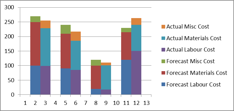
Step-by-step tutorial on creating clustered stacked column bar charts (for free) | Excel Help HQ

How to add Axis Labels (X & Y) in Excel & Google Sheets Adding Axis Labels. Double Click on your Axis; Select Charts & Axis Titles . 3. Click on the Axis Title you want to Change (Horizontal or Vertical Axis) 4. Type in your Title Name . Axis Labels Provide Clarity. Once you change the title for both axes, the user will now better understand the graph.

How To Make A Line Graph In Excel With Multiple Lines On Mac

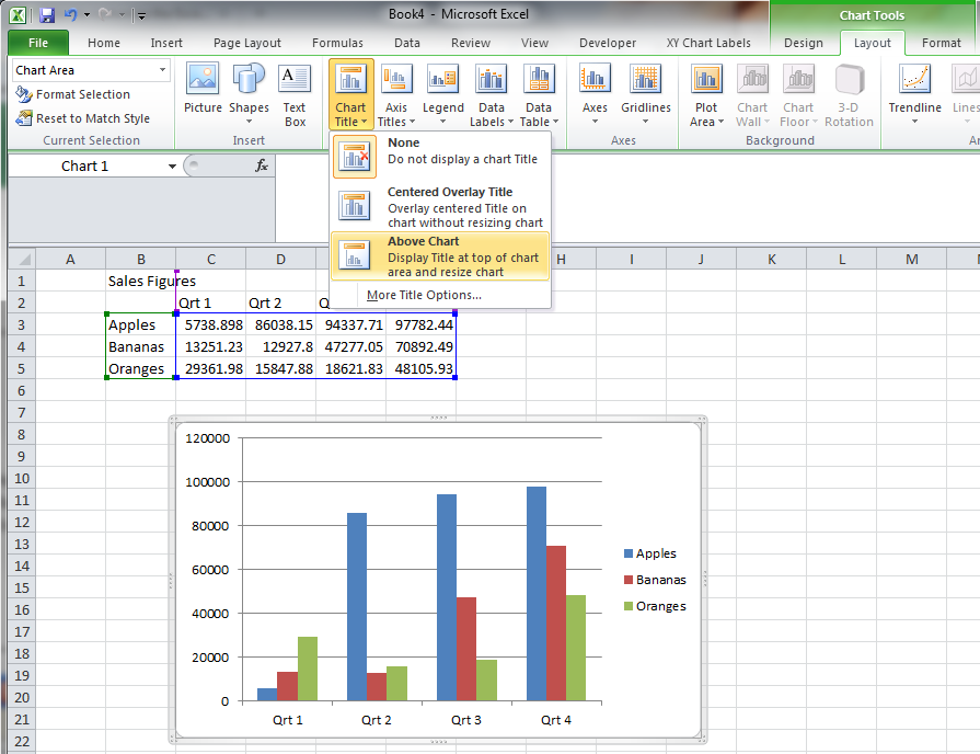
How to Add Axis Titles in a Microsoft Excel Chart Select the chart and go to the Chart Design tab. Click the Add Chart Element drop-down arrow, move your cursor to Axis Titles, and deselect "Primary Horizontal," "Primary Vertical," or both. In Excel on Windows, you can also click the Chart Elements icon and uncheck the box for Axis Titles to remove them both.

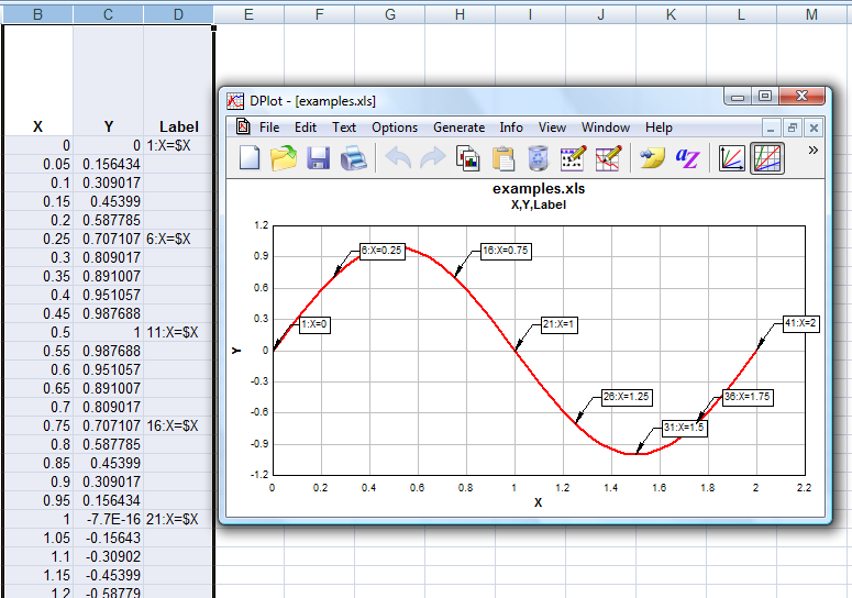
DPlot Windows software for Excel users to create presentation quality graphs

How To Add Axis Labels In Google Sheets in 2022 (+ Examples) A new chart will be inserted and can be edited as needed in the Chart Editor sidebar. Adding Axis Labels. Once you have a chart, it's time to add axis labels: Step 1. Open the Chart Editor by selecting the chart and clicking on the 3 dot menu icon in the corner. From the menu, select Edit Chart. The Chart Editor will open: Step 2. Switch to ...

Link chart title to cell

Text Labels on a Horizontal Bar Chart in Excel - Peltier Tech On the Excel 2007 Chart Tools > Layout tab, click Axes, then Secondary Horizontal Axis, then Show Left to Right Axis. Now the chart has four axes. We want the Rating labels at the bottom of the chart, and we'll place the numerical axis at the top before we hide it. In turn, select the left and right vertical axes.

Axis Labels That Don't Block Plotted Data - Peltier Tech Blog

How to Label Axes in Excel: 6 Steps (with Pictures) - wikiHow Select an "Axis Title" box. Click either of the "Axis Title" boxes to place your mouse cursor in it. Enter a title for the axis. Select the "Axis Title" text, type in a new label for the axis, and then click the graph. This will save your title. You can repeat this process for the other axis title.

r - Breaking value axis using ggplot2 - Stack Overflow

How to Add Axis Labels to a Chart in Excel | CustomGuide Select the set of gridlines you want to show. Add Data Labels Use data labels to label the values of individual chart elements. Select the chart. Click the Chart Elements button. Click the Data Labels check box. In the Chart Elements menu, click the Data Labels list arrow to change the position of the data labels. Display a Data Table

How to Make Your Excel Bar Chart Look Better – MBA Excel

How to Change Excel Chart Data Labels to Custom Values? May 05, 2010 · Col A is x axis labels (hard coded, no spaces in strings, text format), with null cells in between. The labels are every 4 or 5 rows apart with null in between, marking month ends, the data columns are readings taken each week. Y axis is automatic, and works fine. 1050 rows of data for all columns (i.e. 20 years of trend data, and growing).

Share :