44 how to add data labels to a pie chart in excel
Add or remove data labels in a chart - support.microsoft.com Click the data series or chart. To label one data point, after clicking the series, click that data point. In the upper right corner, next to the chart, click Add Chart Element > Data Labels. To change the location, click the arrow, and choose an option. If you want to show your data label inside a text bubble shape, click Data Callout. How to Create and Format a Pie Chart in Excel - Lifewire To add data labels to a pie chart: Select the plot area of the pie chart. Right-click the chart. Select Add Data Labels . Select Add Data Labels. In this example, the sales for each cookie is added to the slices of the pie chart. Change Colors
Possible to add second data label to pie chart? - Excel Help Forum Re: Possible to add second data label to pie chart? Create the composite label in a worksheet column by concatenating the data in other cells and the nextline character, CHR (10). Now, use this composite label column as the source for Rob Bovey's add-in. -- Regards, Tushar Mehta Excel, PowerPoint, and VBA add-ins, tutorials
:max_bytes(150000):strip_icc()/Capture-5c85407246e0fb00010f10e9.JPG)
How to add data labels to a pie chart in excel
How to Create a Pie Chart in Microsoft Excel - template.net How do I add data labels to the pie chart? You first need to select the plot section of the pie chart to add data labels to it. After that, right-click on the chart and click on the Add Data Labels option. Then, choose Add Data Labels once more from the corresponding pop-up options that appear. Edit titles or data labels in a chart - support.microsoft.com On a chart, click one time or two times on the data label that you want to link to a corresponding worksheet cell. The first click selects the data labels for the whole data series, and the second click selects the individual data label. Right-click the data label, and then click Format Data Label or Format Data Labels. Add Labels with Lines in an Excel Pie Chart (with Easy Steps) To enables the data labels on the pie chart, Click on the Pie Chart first. Then click on the plus icon at the top-right corner of the pie chart. Now select Data Labels in the Chart Elements list. After that, you will see a variety of data labels position option such as, Center Inside End Outside End Best Fit Data callout
How to add data labels to a pie chart in excel. How to add data labels from different column in an Excel chart? Right click the data series in the chart, and select Add Data Labels > Add Data Labels from the context menu to add data labels. 2. Click any data label to select all data labels, and then click the specified data label to select it only in the chart. 3. Excel pie chart labels overlap Note that all of the data labels for that data series are selected. Google returns 2. You can add data labels to an Excel 2010 chart to help identify the values shown in each data point of the data series. A bubble pie chart is a bubble chart that uses pie charts instead of bubbles to display multiple levels of data at once. In a single pie. Display data point labels outside a pie chart in a paginated report ... To display data point labels inside a pie chart. Add a pie chart to your report. For more information, see Add a Chart to a Report (Report Builder and SSRS). On the design surface, right-click on the chart and select Show Data Labels. To display data point labels outside a pie chart. Create a pie chart and display the data labels. Open the ... Change the format of data labels in a chart To get there, after adding your data labels, select the data label to format, and then click Chart Elements > Data Labels > More Options. To go to the appropriate area, click one of the four icons ( Fill & Line, Effects, Size & Properties ( Layout & Properties in Outlook or Word), or Label Options) shown here.
How to Edit Pie Chart in Excel (All Possible Modifications) Just like the chart title, you can also change the position of data labels in a pie chart. Follow the steps below to do this. 👇 Steps: Firstly, click on the chart area. Following, click on the Chart Elements icon. Subsequently, click on the rightward arrow situated on the right side of the Data Labels option. How to display leader lines in pie chart in Excel? - ExtendOffice To display leader lines in pie chart, you just need to check an option then drag the labels out. 1. Click at the chart, and right click to select Format Data Labels from context menu. 2. In the popping Format Data Labels dialog/pane, check Show Leader Lines in the Label Options section. See screenshot: 3. Microsoft Excel Tutorials: Add Data Labels to a Pie Chart To add the numbers from our E column (the viewing figures), left click on the pie chart itself to select it: The chart is selected when you can see all those blue circles surrounding it. Now right click the chart. You should get the following menu: From the menu, select Add Data Labels. New data labels will then appear on your chart: How to Make a Pie Chart in Excel - dergipark.railpage.com.au Add a name to the chart. To do so, click the B1 cell and then type in the chart's name.. For example, if you're making a chart about your budget, the B1 cell should say something like "2017 Budget".; You can also type in a clarifying label--e.g., "Budget Allocation"--in the A1A1
How to Make a Pie Chart in Excel & Add Rich Data Labels to The Chart! Formatting the Data Labels of the Pie Chart 1) In cell A11, type the following text, Main reason for unforced errors, and give the cell a light blue fill and a black border. 2) In cell A12, type the text Sinusitis, and give the cell a black border, and align the text to the center position. How to Label a Pie Chart in Excel (6 Steps) - ItStillWorks Clicking on the data series or a specific data point will open the "Chart Tools" tab. Locate the "Labels" group and click on the "Layout" tab. Click the "Data ... Add data labels and callouts to charts in Excel 365 - EasyTweaks.com The steps that I will share in this guide apply to Excel 2021 / 2019 / 2016. Step #1: After generating the chart in Excel, right-click anywhere within the chart and select Add labels . Note that you can also select the very handy option of Adding data Callouts. How to Make a Multi-Level Pie Chart in Excel (with Easy Steps) Step 5: Add Data Labels and Format Them. Adding data labels can help us analyze the information precisely. Right-click on the outermost level on the chart and then right-click on the chart. Then from the context menu, click on the Add Data Labels. After clicking on the Add Data Labels, the data labels will show accordingly.
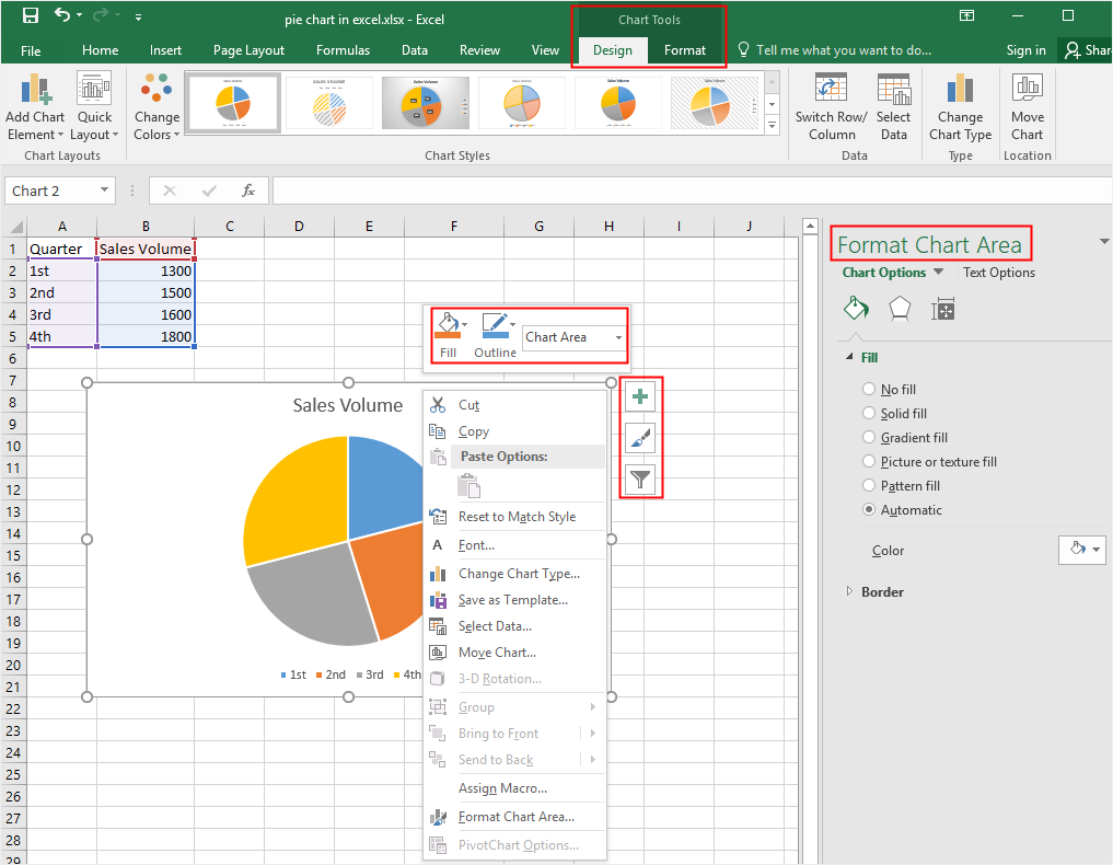
How to Create and Format a Pie Chart in Excel
Add a pie chart - support.microsoft.com Click Insert > Insert Pie or Doughnut Chart, and then pick the chart you want. Click the chart and then click the icons next to the chart to add finishing touches: To show, hide, or format things like axis titles or data labels, click Chart Elements . To quickly change the color or style of the chart, use the Chart Styles .

How to Represent Data with a Pie of Pie Chart in Your Excel Worksheet - Data Recovery Blog
Pie Chart in Excel - Inserting, Formatting, Filters, Data Labels Click on the Instagram slice of the pie chart to select the instagram. Go to format tab. (optional step) In the Current Selection group, choose data series "hours". This will select all the slices of pie chart. Click on Format Selection Button. As a result, the Format Data Point pane opens.
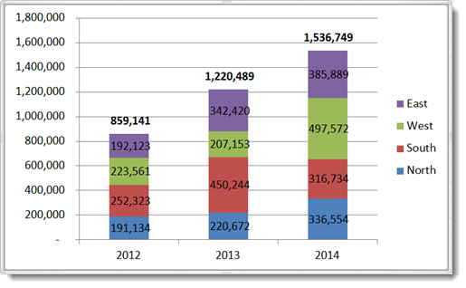
How to Show Percentages in Stacked Bar and Column Charts in Excel
How to Show Pie Chart Data Labels in Percentage in Excel Now we'll add the data labels from the context menu and then will format the data labels in percentages. Steps: Right-click your mouse on any slice of the Pie Chart. After that, select Add Data Labels from the context menu. The data labels are added now, right click on any data label.
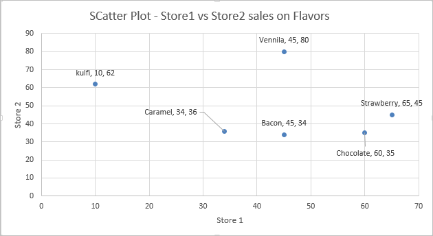
Add Custom Labels to x-y Scatter plot in Excel - DataScience Made Simple
How to show percentage in pie chart in Excel? - ExtendOffice Select the data you will create a pie chart based on, click Insert > I nsert Pie or Doughnut Chart > Pie. See screenshot: 2. Then a pie chart is created. Right click the pie chart and select Add Data Labels from the context menu. 3. Now the corresponding values are displayed in the pie slices.
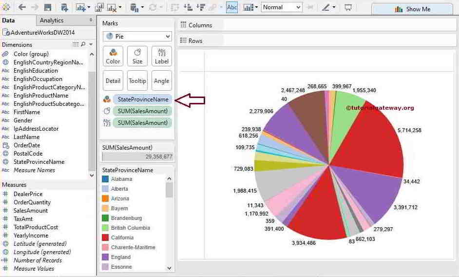
30 Tableau Pie Chart Percentage Label - Label Design Ideas 2020
Pie Chart in Excel | How to Create Pie Chart - EDUCBA Go to the Insert tab and click on a PIE. Step 2: once you click on a 2-D Pie chart, it will insert the blank chart as shown in the below image. Step 3: Right-click on the chart and choose Select Data. Step 4: once you click on Select Data, it will open the below box. Step 5: Now click on the Add button.
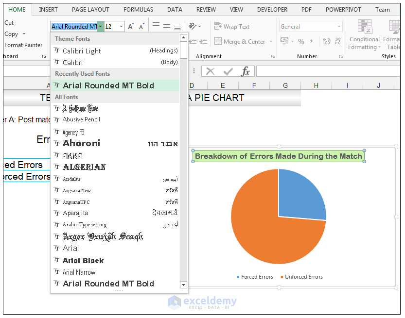
How to Make a Pie Chart in Excel & Add Rich Data Labels to The Chart!
Add Labels with Lines in an Excel Pie Chart (with Easy Steps) To enables the data labels on the pie chart, Click on the Pie Chart first. Then click on the plus icon at the top-right corner of the pie chart. Now select Data Labels in the Chart Elements list. After that, you will see a variety of data labels position option such as, Center Inside End Outside End Best Fit Data callout

How to Create Multi-Category Chart in Excel - Excel Board
Edit titles or data labels in a chart - support.microsoft.com On a chart, click one time or two times on the data label that you want to link to a corresponding worksheet cell. The first click selects the data labels for the whole data series, and the second click selects the individual data label. Right-click the data label, and then click Format Data Label or Format Data Labels.

Excel 2010 pie chart data labels in case of "Best Fit"
How to Create a Pie Chart in Microsoft Excel - template.net How do I add data labels to the pie chart? You first need to select the plot section of the pie chart to add data labels to it. After that, right-click on the chart and click on the Add Data Labels option. Then, choose Add Data Labels once more from the corresponding pop-up options that appear.
How to Make a Pie Chart in Excel & Add Rich Data Labels to The Chart!
How to Make a Pie Chart in Excel & Add Rich Data Labels to The Chart!
How to Make a Pie Chart in Excel | EdrawMax Online
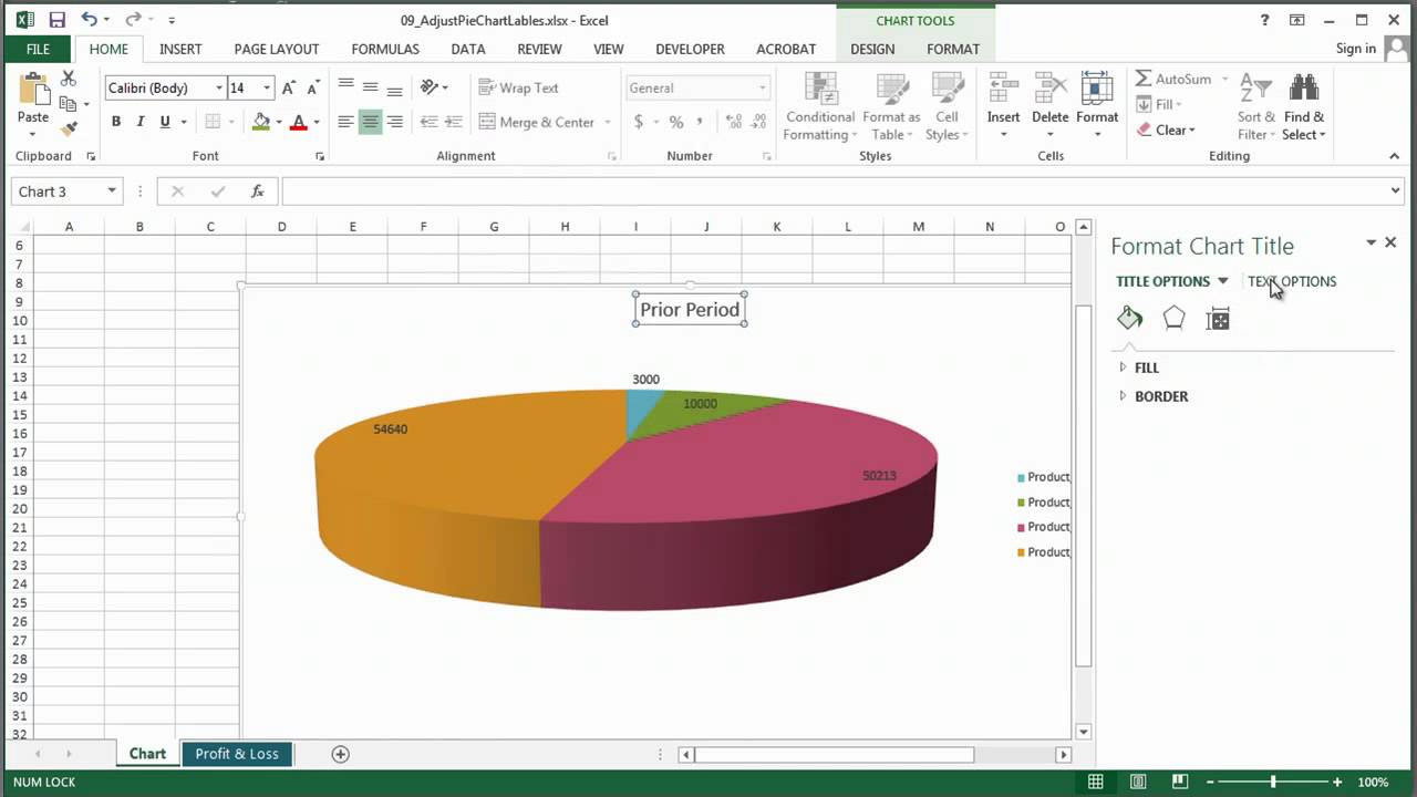
How to Adjust Pie Chart Labels in Excel : MS Excel Tips - YouTube
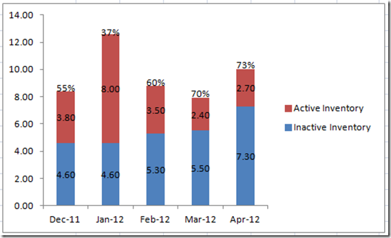
How-to Put Percentage Labels on Top of a Stacked Column Chart - Excel Dashboard Templates

Creating Pie Chart and Adding/Formatting Data Labels (Excel) - YouTube
charts - Showing percentages above bars on Excel column graph - Stack Overflow
Post a Comment for "44 how to add data labels to a pie chart in excel"